Low-lying electronic states
Open shell species of any kind may have a number of different low-lying electronic states that are all self-consistent solutions. Even though DFT is a ground state method, it may be applied directly to the lowest electronic state with well-defined quantum numbers, i.e. the lowest energy or ‘ground state’ of a given angular momentum and spin. All of these low-lying electronic states might seem a bit “exotic”, but this multi-part tutorial on low-lying electronic states should help to demystify them for you!
1. How do I choose my spin?
At the very start, when we describe open-shell species, we should be careful to consider all of the possible spin states the molecule may have.
The total magnetization of a molecule is what is printed in a PWscf calculation and refers to:
tot_magnetization = nelup-neldw
where nelup is typically assumed to be the majority spin. You can determine the maximum total magnetization for a system by adding up all of the unpaired electrons from each atom that comprises your system in any of its’ lowest lying electronic states.
2. Can we bias our solution easily?
It is not necessarily “easy”, but there are a few ways to bias your conditions to try to control which configuration you achieve.
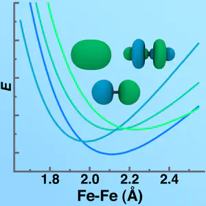
If you know one of your states has more anti-bonding character and another has more bonding character, it may make sense to shorten the bonds in your initial geometry to favor the electronic state that has more bonding character and do the opposite to favor the state with anti-bonding character.
Conversely, if you know that breaking a key bond leads to a higher energy dissociation in one state than another, you may wish to start near dissociation in your geometry. You can then use the density produced at one geometry and slowly change that geometry in order to ensure you remain on the potential energy surface that you want.
One of the best ways to converge multiple low-lying solutions at a single geometry is to change the starting guess via the starting_magnetization keyword (in combination with a spin polarized calculation). Each atom of itype can have a starting_magnetization(i) between -1.0 and 1.0. If this keyword is not set for a given atom type, the code assumes that this atom cannot be spin polarized. In general, if you’re carrying out a spin polarized calculation, I recommend that you set this variable for all atom types even if there are atoms (e.g. hydrogens) that you do not expect to have any spin polarization. Choosing the right guess for starting_magnetization is a bit of a black art, especially if your system has many low-lying solutions. The clearest case is where you are trying to obtain an antiferrogmanetically coupled solution: then you make sure the two antiferromagnetically coupled species (must be different atom types even if they’re the same element) have opposing starting_magnetizations in order to favor this antiferromagnetic coupling.
3. How do I know what my electron configuration is or if the solutions from different calculations are distinct electronic states?
Once you have carried out some calculations on a few different molecules, there are a number of ways to identify your states both on the fly - i.e. as your calculation is running - and through postprocessing after your calculation is complete.
During initial investigations of the low-lying states of a molecule, one may wish to quickly identify the number of different electronic states without any detailed analysis. You can determine two states are distinct if they have significantly different total energies (i.e. more than the convergence threshold of your calculation) or if their absolute magnetization is different despite having the same total magnetization.
Another useful approach is to turn on DFT+U calculations but with a very small value of U (e.g. 1x10⁻¹⁰), even if you don’t intend to use a DFT+U approach, so that an occupation matrix obtained from projections of molecular states onto atomic states is printed in every single point energy or structural relaxation you carry out. In this case, you can put the “zero U” on each atom type that is likely to have significant open shell character - if you have a single site transition metal complex you may only need an occupation matrix on the transition metal.
Finally, the only rigorous approach to identifying electronic states is to enumerate the eigenstates of your molecule either by visualizing each molecular orbital (with pp.x) or through analysis of the projections of these orbitals onto an atomic basis with the projwfc.x code. Although in DFT the eigenvalues and eigenvectors don’t necessarily retain the same meaning as in wavefunction approach, the total angular momentum from the combination of all these individual eigenstates still retains its meaning.
I hope that this tutorial has helped you to better understand how to make the most of identifying low-lying electronic states in Quantum-ESPRESSO and PWscf. Check back here in the coming months for more detailed exploration of low-lying electronic states. Please email me if you have any additional questions not answered here!